Tomorrow's electricity demand
Forecast every hour of tomorrow's electricity demand in Queensland from public AEMO data, issued at 10:00 today, with an 80% range. 23 steps, all shown in full: an issue-time definition with a leakage test, holidays computed from the law, baselines, a 12-month walk-forward backtest, conformal ranges, a weather stress test, an API and accuracy monitoring.
Frame the forecast by when it is issued
A forecast is only defined once you say when it is made and what is known at that moment. Here: at 10:00 on day D, forecast the average demand for every hour of day D+1 in Queensland. At 10:00 you know demand up to 10:00 today, the weather forecast for tomorrow, and the calendar. Nothing else.
| Question | Answer |
|---|---|
| User | An energy retailer hedging tomorrow's purchases (also useful to network planners and analysts) |
| Output | 24 hourly forecasts in MW, each with an 80% range |
| Issue time | 10:00 on day D, market time (AEST: Queensland has no daylight saving, which keeps time simple) |
| Success | Beat "same hour last week" by at least 10%, on a 12-month walk-forward backtest, with ranges that cover about 80% |
| Not for | Operating the grid or bidding into the market in place of AEMO's official forecasts |
docs/problem_framing.md (excerpt)17 lines
## The forecast
| | |
|---|---|
| Target | Mean operational demand (MW) for each hour of day D+1, AEMO region QLD1 |
| Issued | 10:00 on day D, market time (AEST, UTC+10, no daylight saving) |
| Known at issue time | demand up to 10:00 on day D; the weather forecast for day D+1; the calendar |
| Output | 24 point forecasts plus an 80% range |
| Not for | operating the power system or market bidding in place of AEMO's official forecasts |

## Success measures (set before modelling)
| measure | why | threshold |
|---|---|---|
| MAPE on a 12-month walk-forward backtest | standard, scale-free | beat "same hour last week" by ≥ 10% |
| MAE and RMSE (MW) | megawatts are what is bought | reported |
| daily peak error | peaks drive the cost of hedging | reported, with bias |
| 80% range coverage | ranges must mean what they say | 75–85%, also by hour |
| skill with realistic weather-forecast error | production uses forecasts, not observations | reported |configs/config.yaml49 lines
# All settings for the Queensland demand-forecasting project. Change values here, never in code.
project:
  name: demand
  seed: 42

paths:
  raw_dir: data/raw                       # one AEMO CSV per month + weather.csv + PROVENANCE.json
  interim: data/interim/hourly.parquet    # clean hourly demand joined with temperature
  features: data/processed/features.parquet
  model_dir: models
  reports: reports
  runs: runs

data:
  region: QLD1
  first_month: "2019-01"                  # inclusive
  last_month: "2025-12"                   # inclusive
  # AEMO aggregated price and demand data (public; see docs/data_card.md for the terms).
  demand_url: "https://aemo.com.au/aemo/data/nem/priceanddemand/PRICE_AND_DEMAND_{yyyymm}_{region}.csv"
  # Open-Meteo historical weather API (CC BY 4.0). Brisbane: most of Queensland's demand is in the south-east.
  weather_url: "https://archive-api.open-meteo.com/v1/archive"
  latitude: -27.47
  longitude: 153.03
  min_mw: 2500                            # hard limits: outside these, data is wrong (QLD1 runs ~4,000-11,000 MW)
  max_mw: 14000
  max_fill_hours: 3                       # gaps up to this long are interpolated (and flagged); longer gaps stay missing
  extra_holidays: ["2022-09-22"]          # one-off public holidays (National Day of Mourning)

forecast:
  # The forecast is issued at 10:00 on day D for each hour of day D+1 (market time, AEST, no daylight saving).
  # Only demand up to 10:00 on day D may be used; tests enforce this.
  issue_hour: 10

backtest:
  test_months: 12                         # walk-forward over the final 12 months
  refit_every_months: 1                   # refit on all data before each test month
  tuning_folds: 4                         # time-series CV folds on the period before the backtest
  tuning_iterations: 12
  min_gain_over_naive: 0.10               # a model must cut the seasonal-naive MAPE by at least 10%
  temperature_error_c: 1.5                # stress test: simulated weather-forecast error (std, degrees C)
  quantiles: [0.1, 0.9]                   # 80% prediction interval

evaluation:
  bootstrap_samples: 1000

monitoring:
  window_days: 28
  mape_warn_ratio: 1.25                   # recent MAPE vs backtest MAPE
  mape_alert_ratio: 1.5
Reuse the professional repository layout
Same structure and quality gates as Project 1: an installable package, typed config, pinned
dependencies, ruff, strict mypy, pytest, pre-commit, CI and Docker. New here: calendar.py for holidays, and
models/backtest.py, intervals.py and predict.py for the forecasting logic.
Makefile54 lines
# One command per pipeline step. Run `make help` to list them.
PY ?= python
CONFIG ?= configs/config.yaml

.PHONY: help install data synthetic validate prepare eda train evaluate all serve test lint typecheck check clean docker

help:          ## List the available commands
	@grep -E '^[a-z-]+:.*## ' Makefile | sed 's/:.*## /\t/'

install:       ## Install pinned dependencies and the package in editable mode
	$(PY) -m pip install -r requirements-dev.txt && $(PY) -m pip install -e . --no-deps && pre-commit install

data:          ## Download AEMO demand (monthly files) and Open-Meteo temperature, with provenance
	$(PY) -m demand.cli download --config $(CONFIG)

synthetic:     ## Create synthetic AEMO-format files instead (no download needed)
	$(PY) scripts/make_synthetic.py --start 2019-01 --end 2025-12 --raw-dir data/raw

validate:      ## Check the raw files against the schema and physical limits
	$(PY) -m demand.cli validate --config $(CONFIG)

prepare:       ## Hourly series, repairs, temperature, holidays, forecast-time-safe features
	$(PY) -m demand.cli prepare --config $(CONFIG)

eda:           ## Exploratory analysis of the period before the backtest
	$(PY) -m demand.cli eda --config $(CONFIG)

train:         ## Tune, choose, walk-forward backtest, fit the final model
	$(PY) -m demand.cli train --config $(CONFIG)

evaluate:      ## Backtest metrics with intervals, error patterns, the forecast card
	$(PY) -m demand.cli evaluate --config $(CONFIG)

all: validate prepare eda train evaluate   ## Run the whole pipeline

serve:         ## Run the forecast API locally
	$(PY) -m flask --app "demand.serving.app:create_app()" run --debug --port 8000

test:          ## Run the test suite
	$(PY) -m pytest

lint:          ## Lint and check formatting
	ruff check . && ruff format --check .

typecheck:     ## Static type checks
	mypy

check: lint typecheck test   ## Everything CI runs

docker:        ## Build the serving image
	docker build -t demand-api .

clean:         ## Remove generated data, models and reports
	rm -rf data/interim/* data/processed/* models/* reports/* runs/*
Download public data with provenance
Two public sources. AEMO publishes demand for each region of the National Electricity Market as one CSV per month; AEMO allows any use with attribution. Open-Meteo provides historical hourly temperature (CC BY 4.0). The script downloads 84 months politely (with retries and a pause between files) and records every URL and checksum.
src/demand/data/download.py47 lines
def download(cfg: Config, force: bool = False) -> Path:
    """Fetch every month of demand and the matching hourly temperatures; write PROVENANCE.json."""
    d = cfg.data
    raw = cfg.paths.raw_dir
    (raw / "aemo").mkdir(parents=True, exist_ok=True)
    files: dict[str, dict[str, object]] = {}
    for m in d.months:
        path = demand_path(raw, m, d.region)
        url = d.demand_url.format(yyyymm=m.strftime("%Y%m"), region=d.region)
        if force or not path.exists():
            path.write_bytes(_get(url))
            time.sleep(0.5)  # be polite to a public server
        files[path.name] = {"url": url, "sha256": hashlib.sha256(path.read_bytes()).hexdigest()}
    log.info("demand: %d monthly files in %s", len(files), raw / "aemo")

    start = d.months[0].start_time.date()
    end = (
        d.months[-1].end_time + pd.Timedelta(days=1)
    ).date()  # one extra day so every hour has an end temperature
    params = {
        "latitude": d.latitude,
        "longitude": d.longitude,
        "start_date": start,
        "end_date": end,
        "hourly": "temperature_2m",
        "timezone": "Australia/Brisbane",
    }
    wurl = f"{d.weather_url}?{urllib.parse.urlencode(params)}"
    wpath = raw / "weather.csv"
    if force or not wpath.exists():
        js = json.loads(_get(wurl, timeout=180))
        pd.DataFrame(js["hourly"]).to_csv(wpath, index=False)
    files[wpath.name] = {"url": wurl, "sha256": hashlib.sha256(wpath.read_bytes()).hexdigest()}
    prov = {
        "downloaded_at": datetime.now(UTC).isoformat(timespec="seconds"),
        "region": d.region,
        "months": [str(m) for m in d.months],
        "files": files,
        "licences": {
            "AEMO": "AEMO copyright permissions (see docs/data_card.md)",
            "Open-Meteo": "CC BY 4.0, attribution required",
        },
    }
    out = raw / "PROVENANCE.json"
    out.write_text(json.dumps(prov, indent=2), encoding="utf-8")
    log.info("weather: %s; provenance written to %s", wpath.name, out)
    return out
docs/data_card.md: the AEMO columns7 lines
| column | meaning | notes |
|---|---|---|
| REGION | NEM region | always QLD1 here (validated) |
| SETTLEMENTDATE | END of the settlement interval, market time (AEST) | 30-minute intervals until 30 Sep 2021, 5-minute from 1 Oct 2021 |
| TOTALDEMAND | operational demand, MW | excludes demand met by rooftop solar |
| RRP | regional reference price, $/MWh | not used (not known a day ahead) |
| PERIODTYPE | TRADE | |Validate both sources
Hard errors: a missing month, the wrong region, timestamps not in AEMO's format, demand outside physical limits (2,500–14,000 MW for Queensland), the same interval twice with different values, temperatures outside −10 to 50 °C, or weather that does not cover the demand period. Recorded as facts: the switch from 30-minute to 5-minute settlement on 1 October 2021, duplicate rows and gaps.
src/demand/data/schema.py68 lines
def validate(cfg: Config, demand: pd.DataFrame, weather: pd.DataFrame) -> ValidationReport:
    """Check both sources against the schema and physical limits."""
    rep = ValidationReport()
    d = cfg.data
    missing_files = [str(m) for m in d.months if not demand_path(cfg.paths.raw_dir, m, d.region).exists()]
    if missing_files:
        rep.errors.append(f"missing AEMO months: {missing_files}")
    miss = [c for c in DEMAND_COLUMNS if c not in demand.columns]
    if miss:
        rep.errors.append(f"demand file missing columns {miss}")
        return rep
    regions = set(demand["REGION"].astype(str).unique())
    if regions != {d.region}:
        rep.errors.append(f"expected only region {d.region}, found {sorted(regions)}")
    ts = pd.to_datetime(demand["SETTLEMENTDATE"], format="%Y/%m/%d %H:%M:%S", errors="coerce")
    if ts.isna().any():
        rep.errors.append(f"{int(ts.isna().sum())} SETTLEMENTDATE values not like 2024/01/31 13:05:00")
    mw = pd.to_numeric(demand["TOTALDEMAND"], errors="coerce")
    if mw.isna().any():
        rep.errors.append(f"{int(mw.isna().sum())} missing or non-numeric TOTALDEMAND values")
    out_of_range = ((mw < d.min_mw) | (mw > d.max_mw)).sum()
    if out_of_range:
        rep.errors.append(f"{int(out_of_range)} demand values outside {d.min_mw:.0f}-{d.max_mw:.0f} MW")
    dup = demand.duplicated(subset=["REGION", "SETTLEMENTDATE"], keep=False)
    conflicting = demand[dup].groupby("SETTLEMENTDATE")["TOTALDEMAND"].nunique().gt(1).sum()
    if conflicting:
        rep.errors.append(f"{int(conflicting)} timestamps appear twice with different demand values")
    step = ts.sort_values().diff().dt.total_seconds().div(60)
    rep.facts.update(
        {
            "rows": len(demand),
            "first": str(ts.min()),
            "last": str(ts.max()),
            "exact_duplicates": int(demand.duplicated().sum()),
            "intervals_30min": int((step == 30).sum()),
            "intervals_5min": int((step == 5).sum()),
            "gaps_over_1h": int((step > 60).sum()),
            "demand_mean_mw": round(float(mw.mean()), 1),
        }
    )
    if rep.facts["exact_duplicates"]:
        rep.warnings.append(f"{rep.facts['exact_duplicates']} exact duplicate rows (removed in prepare)")
    if rep.facts["gaps_over_1h"]:
        rep.warnings.append(
            f"{rep.facts['gaps_over_1h']} gaps longer than an hour "
            "(short ones filled, long ones left missing)"
        )

    wmiss = [c for c in WEATHER_COLUMNS if c not in weather.columns]
    if wmiss:
        rep.errors.append(f"weather file missing columns {wmiss}")
        return rep
    wt = pd.to_datetime(weather["time"], errors="coerce")
    temp = pd.to_numeric(weather["temperature_2m"], errors="coerce")
    if wt.isna().any():
        rep.errors.append("unparseable weather times")
    if ((temp < -10) | (temp > 50)).any():
        rep.errors.append("temperatures outside -10..50 degrees C")
    if (
        not ts.isna().all()
        and not wt.isna().all()
        and (wt.min() > ts.min() or wt.max() < ts.max() - pd.Timedelta(hours=1))
    ):
        rep.errors.append("weather does not cover the whole demand period")
    rep.facts["weather_missing_hours"] = int(temp.isna().sum())
    if rep.facts["weather_missing_hours"]:
        rep.warnings.append(f"{rep.facts['weather_missing_hours']} hours without temperature (interpolated)")
return repBuild a clean hourly series
AEMO timestamps mark the end of each interval. So the interval ending at 01:00 belongs to the hour starting at 00:00, and the interval ending at 00:05 does too. Getting this wrong shifts every value by one interval and quietly damages every lag. Hourly demand is the mean MW of the intervals in the hour, which works for both 30- and 5-minute data.
src/demand/data/prepare.py9 lines
def to_hourly(demand: pd.DataFrame) -> pd.DataFrame:
    """Mean demand per hour (hour-starting index) and how many intervals it was built from."""
    df = demand.drop_duplicates(subset=["REGION", "SETTLEMENTDATE"]).copy()
    end = pd.to_datetime(df["SETTLEMENTDATE"], format="%Y/%m/%d %H:%M:%S")
    hour = (end - pd.Timedelta(seconds=1)).dt.floor("h")  # interval ending 01:00 belongs to hour 00:00
    g = pd.to_numeric(df["TOTALDEMAND"]).groupby(hour)
    out = pd.DataFrame({"demand_mw": g.mean(), "n_intervals": g.size()})
    out.index.name = "ts"
    return out
tests/test_data.py: the convention, tested9 lines
def test_interval_ending_timestamps_map_to_the_hour_they_end_in() -> None:
    ends = [f"2024/01/01 00:{m:02d}:00" for m in range(5, 60, 5)] + [
        "2024/01/01 01:00:00",
        "2024/01/01 01:05:00",
    ]
    h = to_hourly(_rows(ends, [100.0] * 11 + [160.0, 999.0]))
    assert h.loc["2024-01-01 00:00", "demand_mw"] == pytest.approx(105.0)  # mean of eleven 100s and one 160
    assert h.loc["2024-01-01 00:00", "n_intervals"] == 12
assert h.loc["2024-01-01 01:00", "n_intervals"] == 1Repair short gaps, leave long ones missing
Gaps of up to 3 hours are interpolated and flagged; longer gaps stay missing, and those hours are dropped from training and evaluation
rather than filled with invented numbers. Every count goes into reports/prepare_log.json.
src/demand/data/prepare.py: gap rules10 lines
filled = df["demand_mw"].interpolate(method="time", limit=cfg.data.max_fill_hours, limit_area="inside")
# interpolate(limit=...) fills the first hours of a long gap too; undo that so long gaps stay missing.
run_id = missing.ne(missing.shift()).cumsum()
run_len = missing.groupby(run_id).transform("sum")
long_gap = missing & (run_len > cfg.data.max_fill_hours)
filled[long_gap] = float("nan")
df["imputed"] = (missing & filled.notna()).astype("int8")
df["demand_mw"] = filled
plog.counts["hours_interpolated"] = int(df["imputed"].sum())
plog.counts["hours_left_missing"] = int(df["demand_mw"].isna().sum())Compute public holidays from the law
Holidays look like Sundays in the data. Instead of adding a dependency, the Queensland rules (Holidays Act 1983) are coded directly: Easter by the standard algorithm, "first Monday of May", and the substitute days when Christmas or New Year fall on a weekend. One-off holidays, such as the 2022 National Day of Mourning, come from the config.
src/demand/calendar.py25 lines
def qld_holidays(year: int) -> dict[date, str]:
    """State-wide Queensland public holidays for one year (2017 onwards rules)."""
    e = easter_sunday(year)
    h: dict[date, str] = {
        _next_monday_if_weekend(date(year, 1, 1)): "New Year's Day",
        _next_monday_if_weekend(date(year, 1, 26)): "Australia Day",
        e - timedelta(days=2): "Good Friday",
        e - timedelta(days=1): "Easter Saturday",
        e: "Easter Sunday",
        e + timedelta(days=1): "Easter Monday",
        date(year, 4, 25): "Anzac Day",
        _first_monday(year, 5): "Labour Day",
        _first_monday(year, 10): "King's Birthday" if year >= 2023 else "Queen's Birthday",
        date(year, 12, 25): "Christmas Day",
        date(year, 12, 26): "Boxing Day",
    }
    xmas = date(year, 12, 25)
    if xmas.weekday() == 5:  # Saturday: Monday 27th and Tuesday 28th are added
        h[date(year, 12, 27)] = "Christmas Day (additional)"
        h[date(year, 12, 28)] = "Boxing Day (additional)"
    elif xmas.weekday() == 6:  # Sunday: Boxing Day is Monday; Tuesday 27th is added
        h[date(year, 12, 27)] = "Christmas Day (additional)"
    elif xmas.weekday() == 4:  # Friday: Boxing Day is Saturday; Monday 28th is added
        h[date(year, 12, 28)] = "Boxing Day (additional)"
    return h
tests: checked against the official 2024 list15 lines
def test_qld_2024_matches_the_official_list() -> None:
    expected = {
        date(2024, 1, 1),
        date(2024, 1, 26),
        date(2024, 3, 29),
        date(2024, 3, 30),
        date(2024, 3, 31),
        date(2024, 4, 1),
        date(2024, 4, 25),
        date(2024, 5, 6),
        date(2024, 10, 7),
        date(2024, 12, 25),
        date(2024, 12, 26),
    }
assert set(qld_holidays(2024)) == expectedExplore the years before the backtest
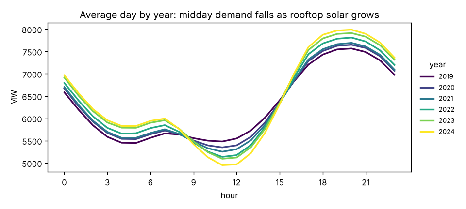
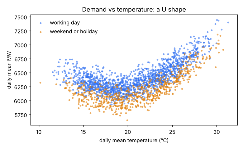
EDA uses only data before the backtest period. Four findings shape the model:
- A U-shape with temperature: demand rises on hot days (air-conditioning) and, less, on cold mornings; weekends sit lower.
- The duck curve: AEMO's operational demand excludes what rooftop solar supplies, so midday demand falls year after year while the evening peak grows.
- Strong daily and weekly memory, but lags shorter than 37 hours cannot be used for every target hour.
- Holidays and weekends behave alike.
Build features from the issue time
For a target hour on day D+1: lags of 48 h, 168 h and 336 h (always fully known), the mean of the same hour over the last four weeks, yesterday's mean, the latest observation (09:00 today) and this morning's level compared with yesterday morning, calendar features, and temperature turned into cooling and heating degrees. One function builds features for training, backtesting and the API.
src/demand/features/build.py40 lines
def build_features(hourly: pd.DataFrame, issue_hour: int) -> pd.DataFrame:
    """One row per hour of ``hourly`` with every feature and the target (NaN where unknown).

    ``hourly`` needs columns ts, demand_mw, temp_c, is_holiday on a complete hourly index.
    """
    df = hourly.set_index("ts").sort_index()
    if not (df.index.to_series().diff().dropna() == pd.Timedelta(hours=1)).all():
        raise ValueError("build_features needs a complete hourly index (no missing or repeated hours)")
    y = df[TARGET]
    idx = df.index
    f = pd.DataFrame(index=idx)
    f["hour"] = idx.hour
    f["dow"] = idx.dayofweek
    f["is_holiday"] = df["is_holiday"].astype("int8").to_numpy()
    f["is_day_off"] = ((idx.dayofweek >= 5) | (f["is_holiday"] == 1)).astype("int8")
    doy = idx.dayofyear.to_numpy()
    f["doy_sin"], f["doy_cos"] = np.sin(2 * np.pi * doy / 365.25), np.cos(2 * np.pi * doy / 365.25)
    f["t_years"] = (idx - EPOCH).total_seconds() / (365.25 * 86400)

    f["lag_48h"] = y.shift(48)
    f["lag_168h"] = y.shift(168)
    f["lag_336h"] = y.shift(336)
    f["ref_4w"] = (y.shift(168) + y.shift(336) + y.shift(504) + y.shift(672)) / 4

    daily_mean = y.groupby(idx.normalize()).mean()
    target_day = idx.normalize()
    f["prev_day_mean"] = daily_mean.reindex(target_day - pd.Timedelta(days=2)).to_numpy()  # day D-1: complete

    issue_day = target_day - pd.Timedelta(days=1)  # day D
    f["latest_obs"] = y.reindex(issue_day + pd.Timedelta(hours=issue_hour - 1)).to_numpy()
    morning = y[idx.hour < issue_hour].groupby(idx[idx.hour < issue_hour].normalize()).mean()
    f["morning_mean"] = morning.reindex(issue_day).to_numpy()
    f["morning_change"] = f["morning_mean"] - morning.reindex(issue_day - pd.Timedelta(days=1)).to_numpy()

    w = weather_features(df["temp_c"], idx)
    for c in WEATHER:
        f[c] = w[c].to_numpy()
    f[TARGET] = y
    f.index.name = "ts"
return f[FEATURES + [TARGET]]Prove there is no leakage
The strongest test in the project: multiply every demand value from 10:00 on day D onwards by three, rebuild the features, and check that the features for day D+1 have not changed at all. If anyone later adds a feature that peeks past the issue time, this test fails.
tests/test_features.py9 lines
def test_no_information_after_the_issue_time_is_used(hourly: pd.DataFrame) -> None:
    """Change every value at or after 10:00 on day D: the features for day D+1 must not move."""
    target = pd.Timestamp("2024-04-17")
    issue = target - pd.Timedelta(days=1) + pd.Timedelta(hours=ISSUE)
    before = build_features(hourly, ISSUE).loc[target : target + pd.Timedelta(hours=23), FEATURES]
    tampered = hourly.copy()
    tampered.loc[tampered["ts"] >= issue, "demand_mw"] *= 3
    after = build_features(tampered, ISSUE).loc[target : target + pd.Timedelta(hours=23), FEATURES]
pd.testing.assert_frame_equal(before, after)Start with baselines
Two baselines that cost nothing: same hour last week (captures the daily and weekly cycle) and the mean of the same hour over the last four weeks (smoother). Any model must cut the first one's error by at least 10% to be released.
src/demand/models/pipelines.py4 lines
def naive(name: str, X: pd.DataFrame) -> npt.NDArray[np.float64]:
    """Baselines: same hour last week, or the mean of the same hour over the last four weeks."""
    col = {"naive_7d": "lag_168h", "naive_4w": "ref_4w"}[name]
return np.asarray(X[col].to_numpy(dtype=float), dtype=float)Model the change, not the level
Tree models cannot predict values outside what they saw in training, and demand drifts over the years. The fix is to let every model predict the difference from the four-week reference and add it back. The trees then only need to learn how tomorrow differs from recent weeks: hotter, a holiday, a Monday.
src/demand/models/pipelines.py17 lines
class OffsetRegressor(BaseEstimator, RegressorMixin):  # type: ignore[misc]
    """Fit ``estimator`` on ``y - X[offset]`` and add ``X[offset]`` back when predicting."""

    def __init__(self, estimator: Any, offset: str = REFERENCE) -> None:
        self.estimator = estimator
        self.offset = offset

    def fit(self, X: pd.DataFrame, y: pd.Series) -> OffsetRegressor:
        """Fit the inner estimator on the difference from the reference level."""
        self.estimator_ = clone(self.estimator).fit(X, np.asarray(y) - X[self.offset].to_numpy())
        return self

    def predict(self, X: pd.DataFrame) -> npt.NDArray[np.float64]:
        """Predicted demand in MW."""
        inner = np.asarray(self.estimator_.predict(X), dtype=float)
        offset = np.asarray(X[self.offset].to_numpy(dtype=float), dtype=float)
return inner + offsetTwo candidates: ridge with splines, gradient boosting
Ridge regression with hour × working-day dummies (the shape of the day), temperature splines and scaled lags.
Gradient boosting with hour and weekday as categorical features. Both are tuned with TimeSeriesSplit on the years
before the backtest, and the model is chosen on that score.
src/demand/models/pipelines.py: the linear model38 lines
def ridge_pipeline(alpha: float = 1.0) -> Pipeline:
    """Linear model: daily-profile dummies, temperature splines, seasonal splines, scaled lags."""
    numeric = [
        "lag_48h",
        "lag_168h",
        "lag_336h",
        "ref_4w",
        "prev_day_mean",
        "latest_obs",
        "morning_mean",
        "morning_change",
        "t_years",
        "is_holiday",
    ]
    pre = ColumnTransformer(
        [
            (
                "profile",
                Pipeline(
                    [
                        ("cross", FunctionTransformer(_hour_daytype, feature_names_out=_hour_daytype_names)),
                        ("onehot", OneHotEncoder(handle_unknown="ignore", sparse_output=False)),
                    ]
                ),
                ["hour", "is_day_off"],
            ),
            ("dow", OneHotEncoder(handle_unknown="ignore", sparse_output=False), ["dow"]),
            (
                "temp",
                SplineTransformer(n_knots=8, degree=3, extrapolation="linear"),
                ["temp_c", "day_max_temp"],
            ),
            ("season", "passthrough", ["doy_sin", "doy_cos"]),
            ("num", StandardScaler(), numeric),
        ],
        verbose_feature_names_out=False,
    )
    return Pipeline([("pre", pre), ("model", Ridge(alpha=alpha))])
src/demand/models/train.py: tuning before the backtest24 lines
def tune(pre: pd.DataFrame, cfg: Config) -> tuple[dict[str, dict[str, Any]], dict[str, float]]:
    """Best parameters and cross-validated MAPE per candidate, on the pre-backtest period only."""
    b = cfg.backtest
    cv = TimeSeriesSplit(n_splits=b.tuning_folds, test_size=min(24 * 56, len(pre) // (b.tuning_folds + 1)))
    X, y = pre[FEATURES], pre[TARGET]
    best: dict[str, dict[str, Any]] = {}
    scores: dict[str, float] = {}
    naive_cv = float(np.mean([mape(y.iloc[te], naive("naive_7d", X.iloc[te])) for _, te in cv.split(X)]))
    scores["naive_7d"] = naive_cv
    for name in CANDIDATES:
        search = RandomizedSearchCV(
            build(name, seed=cfg.project.seed),
            search_space(name),
            n_iter=b.tuning_iterations,
            cv=cv,
            scoring="neg_mean_absolute_percentage_error",
            random_state=cfg.project.seed,
            n_jobs=-1,
        )
        search.fit(X, y)
        best[name], scores[name] = _strip(search.best_params_), float(-search.best_score_)
        log.info("%s: CV MAPE %.2f%% with %s", name, 100 * scores[name], best[name])
    log.info("seasonal naive CV MAPE %.2f%%", 100 * naive_cv)
return best, scoresBacktest walk-forward over a full year
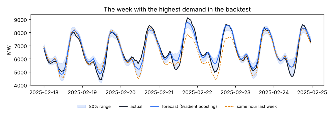
For each of the final 12 months: train on everything before it, forecast it, move on. This is exactly how the model will be used, it covers every season, and the backtest is never used to choose anything.
src/demand/models/backtest.py9 lines
def make_folds(last_ts: pd.Timestamp, test_months: int, refit_every: int) -> list[Fold]:
    """Monthly walk-forward folds covering the final ``test_months`` months of data."""
    last_month = last_ts.to_period("M")
    months = pd.period_range(last_month - test_months + 1, last_month, freq="M")
    folds = []
    for i in range(0, len(months), refit_every):
        chunk = months[i : i + refit_every]
        folds.append(Fold(chunk[0].start_time, (chunk[-1] + 1).start_time))
return folds| Model (synthetic data) | MAPE | MAE (MW) | skill vs last week |
|---|---|---|---|
| Same hour last week | 5.14% | 306 | +0% |
| Mean of last 4 weeks | 4.15% | 247 | +19% |
| Ridge | 3.34% | 192 | +35% |
| Gradient boosting | 3.19% | 184 | +38% |
Calibrate the ranges with conformal prediction
Quantile gradient boosting gives a 10th–90th percentile range, but on its own it covered only about two thirds of actual values, not 80%. Conformalized quantile regression fixes this: fit the quantile models on all but the last 8 weeks of training data, measure on those 8 weeks how far actuals fall outside the range, and widen every future range by that amount. Backtest coverage after calibration: 79.9%.
src/demand/models/intervals.py68 lines
"""Prediction ranges by conformalized quantile regression (CQR).

Quantile gradient boosting alone usually gives ranges that are too narrow (it fits the training data
closely). CQR fixes that with a calibration window the quantile models did not see: measure how far
actuals fall outside the raw range there, and widen every future range by that amount (Romano et al., 2019).
For time series the calibration window is the most recent stretch of training data, which also keeps
the correction up to date.
"""

from __future__ import annotations

from dataclasses import dataclass
from typing import Any

import numpy as np
import numpy.typing as npt
import pandas as pd

from demand.models.pipelines import OffsetRegressor, hgb_estimator


@dataclass
class IntervalModel:
    """Lower and upper quantile models plus the conformal widening ``qhat`` (MW)."""

    lower: OffsetRegressor
    upper: OffsetRegressor
    qhat: float
    target_coverage: float

    def predict(self, X: pd.DataFrame) -> tuple[npt.NDArray[np.float64], npt.NDArray[np.float64]]:
        """Return (lower, upper) in MW, never crossing."""
        lo = self.lower.predict(X) - self.qhat
        hi = self.upper.predict(X) + self.qhat
        return np.minimum(lo, hi), np.maximum(lo, hi)


def conformal_qhat(scores: npt.ArrayLike, coverage: float) -> float:
    """Return the finite-sample conformal quantile of the conformity scores."""
    s = np.sort(np.asarray(scores, dtype=float))
    n = len(s)
    k = min(n, int(np.ceil((n + 1) * coverage)))
    return float(s[k - 1])


def fit_intervals(
    X: pd.DataFrame,
    y: pd.Series,
    quantiles: tuple[float, float],
    hgb_params: dict[str, Any],
    cal_hours: int,
    seed: int,
) -> IntervalModel:
    """Fit quantile models on all but the last ``cal_hours`` rows, calibrate on those rows."""
    fit_X, fit_y, cal_X, cal_y = (
        X.iloc[:-cal_hours],
        y.iloc[:-cal_hours],
        X.iloc[-cal_hours:],
        y.iloc[-cal_hours:],
    )
    lower, upper = (
        OffsetRegressor(hgb_estimator(loss="quantile", quantile=q, seed=seed, **hgb_params)).fit(fit_X, fit_y)
        for q in quantiles
    )
    yc = cal_y.to_numpy()
    scores = np.maximum(lower.predict(cal_X) - yc, yc - upper.predict(cal_X))
    target = quantiles[1] - quantiles[0]
    return IntervalModel(lower, upper, conformal_qhat(scores, target), target)
Stress-test with weather-forecast error
The backtest uses observed temperature, which a real forecaster does not have at 10:00 the day before. So the backtest is repeated with simulated forecast error: a daily error of 1.5 °C plus hourly noise. On the synthetic data MAPE rises from 3.19% to 3.56%. Both numbers go in the forecast card: production accuracy will sit between them.
src/demand/features/build.py10 lines
def perturb_temperature(X: pd.DataFrame, sd: float, rng: np.random.Generator) -> pd.DataFrame:
    """Simulate weather-forecast error: a per-day error plus a smaller hourly one, then rebuild features."""
    days = X.index.normalize()
    codes, uniq = pd.factorize(days)
    err = rng.normal(0, sd, len(uniq))[codes] + rng.normal(0, sd / 3, len(X))
    out = X.copy()
    w = weather_features(X["temp_c"] + err, X.index)
    for c in WEATHER:
        out[c] = w[c].to_numpy()
return outFind where it struggles
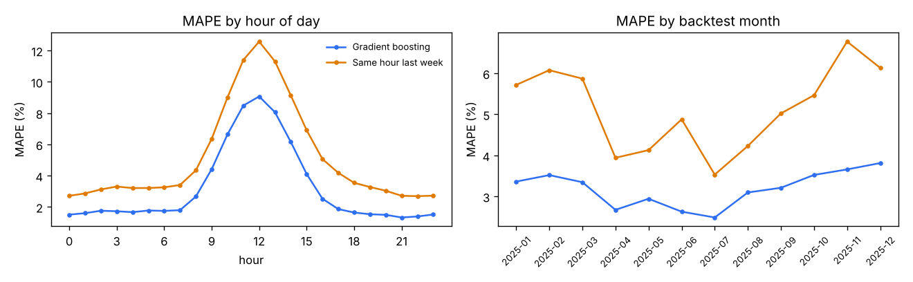
Average error hides the hours that matter. Break errors down by hour of day, month, day type (working day, weekend, public holiday) and look at the daily peak separately, with its bias. The worst days are listed in the card for investigation.
Write the forecast card
Generated by make evaluate: what is forecast and when, how the model was chosen, backtest accuracy with bootstrap
intervals (resampling whole days, because hours within a day are correlated), the weather stress test, range coverage, weak spots,
drivers, limitations and how to operate it.
src/demand/evaluation/metrics.py: bootstrap over days14 lines
def day_bootstrap(
    ts: pd.DatetimeIndex, stat: Callable[[npt.NDArray[np.int_]], float], n: int, seed: int
) -> tuple[float, float]:
    """95% interval for ``stat(rows)`` resampling whole days (hours within a day are correlated)."""
    days = ts.normalize()
    codes, uniq = pd.factorize(days)
    rows_by_day = [np.flatnonzero(codes == i) for i in range(len(uniq))]
    rng = np.random.default_rng(seed)
    vals = []
    for _ in range(n):
        pick = rng.integers(0, len(uniq), len(uniq))
        vals.append(stat(np.concatenate([rows_by_day[i] for i in pick])))
    lo, hi = np.percentile(vals, [2.5, 97.5])
return float(lo), float(hi)Test the time logic hardest
46 tests. The time logic gets the most: the interval-ending convention, 30- and 5-minute data, gap rules, holiday rules and substitute days, the leakage test, lags pointing at the right hours, walk-forward folds, conformal coverage on simulated data, an end-to-end run, API contract tests, training-serving parity, and a monitoring alert.
tests/test_pipeline_and_api.py8 lines
def test_values_after_the_issue_time_are_ignored(client: FlaskClient, trained: Config) -> None:
    body = _body(trained)
    base = client.post("/v1/forecast", json=body).get_json()["forecasts"]
    for o in body["history"]:
        if o["ts"] >= f"{pd.Timestamp(TARGET_DAY) - pd.Timedelta(hours=14):%Y-%m-%dT%H}":
            o["demand_mw"] = 19_000.0
    again = client.post("/v1/forecast", json=body).get_json()["forecasts"]
assert [f["demand_mw"] for f in again] == [f["demand_mw"] for f in base]Serve tomorrow's forecast
POST /v1/forecast takes at least 28 days of hourly history and tomorrow's 24 temperatures, checks the history has no gaps
in the hours the features need, ignores anything after the issue time, and returns 24 forecasts with ranges plus an
out_of_period flag when the model is more than six months old.
src/demand/models/predict.py35 lines
def forecast_day(
    bundle: dict[str, Any], history: pd.Series, target: date, temps_c: list[float]
) -> pd.DataFrame:
    """Hourly forecast and range for ``target`` from hour-starting ``history`` (MW) and 24 temperatures."""
    first, issue = required_window(target, bundle["issue_hour"])
    day = pd.Timestamp(target)
    idx = pd.date_range(first, day + pd.Timedelta(hours=23), freq="h", name="ts")
    hist = history[~history.index.duplicated(keep="last")]
    demand = hist.reindex(idx)
    demand[idx >= issue] = np.nan  # anything at or after the issue time is ignored, never used
    gaps = demand[(idx >= first) & (idx < issue)].isna()
    if gaps.any():
        raise HistoryError(
            f"history is missing {int(gaps.sum())} of the hours "
            f"from {first} to {issue - pd.Timedelta(hours=1)}"
        )
    temp = pd.Series(np.nan, index=idx)
    temp[idx >= day] = temps_c
    hol = holiday_dates(idx[0], idx[-1], bundle["extra_holidays"])
    frame = pd.DataFrame(
        {
            "ts": idx,
            TARGET: demand.to_numpy(),
            "temp_c": temp.to_numpy(),
            "is_holiday": pd.Index(idx.date).isin(hol).astype("int8"),
        }
    )
    X = build_features(frame, bundle["issue_hour"]).loc[day:, FEATURES]
    check_features(X)
    if X.isna().any().any():
        raise HistoryError("could not build every feature from the history provided")
    point = bundle["model"].predict(X)
    lo, hi = bundle["intervals"].predict(X)
    lo, hi = np.minimum(lo, point), np.maximum(hi, point)  # a range must contain its own point forecast
return pd.DataFrame({"demand_mw": point, "lower_mw": lo, "upper_mw": hi}, index=X.index)src/demand/serving/schemas.py16 lines
class ForecastRequest(BaseModel):
    """Forecast every hour of ``target_date`` from recent history and the temperature forecast."""

    model_config = ConfigDict(extra="forbid")
    target_date: date
    history: list[Observation] = Field(min_length=24 * 28, max_length=24 * 60)
    temperature_forecast_c: list[float] = Field(
        min_length=24, max_length=24, description="hours 00..23 of target_date"
    )

    @field_validator("temperature_forecast_c")
    @classmethod
    def _plausible(cls, v: list[float]) -> list[float]:
        if any(not -10 <= t <= 50 for t in v):
            raise ValueError("temperatures must be between -10 and 50 degrees C")
return vDocker and CI
The same production Dockerfile and GitHub Actions workflow as Project 1; CI runs the whole pipeline on two years of synthetic data.
.github/workflows/ci.yml28 lines
name: ci
on:
  push:
  pull_request:

jobs:
  check:
    runs-on: ubuntu-latest
    steps:
      - uses: actions/checkout@v4
      - uses: actions/setup-python@v5
        with:
          python-version: "3.12"
          cache: pip
      - name: Install
        run: |
          python -m pip install -r requirements-dev.txt
          python -m pip install -e . --no-deps
      - name: Lint
        run: ruff check . && ruff format --check .
      - name: Type check
        run: mypy
      - name: Tests (synthetic data, no download needed)
        run: python -m pytest --cov=demand --cov-report=term-missing
      - name: Pipeline smoke run on synthetic data
        run: |
          python scripts/make_synthetic.py --start 2023-01 --end 2024-12 --raw-dir data/raw
          make all CONFIG=configs/ci.yaml
Monitor accuracy, refit monthly
For a forecast, the truth arrives the next day, so monitor accuracy directly: 28-day MAPE against the backtest MAPE (alert at 1.5×), bias, and coverage. Input drift is reported as context. Refit monthly, which is what the backtest measured.
src/demand/monitoring/drift.py28 lines
def accuracy_report(
    bundle: dict[str, Any], feats: pd.DataFrame, window_days: int, warn: float, alert: float
) -> dict[str, Any]:
    """Forecast the last ``window_days`` days that have actuals and compare MAPE with the backtest MAPE."""
    rows = training_rows(feats)
    end = rows.index.max().normalize() + pd.Timedelta(days=1)
    recent = rows[rows.index >= end - pd.Timedelta(days=window_days)]
    year = pd.Timedelta(days=364)  # 52 weeks: same weekdays, same season
    ref = rows[(rows.index >= recent.index.min() - year) & (rows.index <= recent.index.max() - year)]
    pred = bundle["model"].predict(recent[FEATURES])
    m = mape(recent[TARGET], pred)
    ratio = m / bundle["backtest_mape"]
    status = "alert" if ratio >= alert else "warn" if ratio >= warn else "ok"
    drift = (
        {c: round(psi(ref[c], recent[c]), 3) for c in ("temp_c", "latest_obs", "ref_4w")}
        if len(ref) > 100
        else {}
    )
    return {
        "window": [str(recent.index.min()), str(recent.index.max())],
        "hours": len(recent),
        "mape": m,
        "backtest_mape": bundle["backtest_mape"],
        "ratio": ratio,
        "bias_mw": bias(recent[TARGET], pred),
        "status": status,
        "input_psi_vs_same_weeks_last_year": drift,
}docs/monitoring.md18 lines
# Monitoring plan

| what | how | when | action |
|---|---|---|---|
| accuracy | MAPE over the last 28 days vs the backtest MAPE | daily | warn at 1.25×, alert at 1.5× |
| bias | mean forecast minus actual (MW), last 28 days | daily | investigate if above 2% of mean demand |
| range coverage | share of actuals inside the 80% range | weekly | recalibrate if outside 70–90% |
| inputs | PSI of temperature, latest demand and the 4-week reference vs the same weeks last year | weekly | context for accuracy alerts |
| API | latency, 4xx/5xx rate, `out_of_period` responses | continuous | page on 5xx > 1% |

```bash
python -m demand.cli monitor --hourly data/interim/latest.parquet   # exit code 2 = alert
```
Run it only on hours the model was not trained on: in-sample hours look better than reality.

**Refit:** monthly with the latest data (the backtest already refits monthly, so this matches what was measured).
Keep the previous bundle; roll back if the new one is worse on the last month. Add new one-off public holidays to the
config before they happen.
Present it in your portfolio
- Lead with the peak-week chart and the backtest table against the two baselines.
- Explain the issue time and show the leakage test: it is the question interviewers ask about any time-series project.
- Mention the duck curve, conformal ranges and the weather stress test; they show you understand the domain, not just the library.